
What is the fiscal multiplier and why is it so controversial?
Exploring Economics, 2020
What is the fiscal multiplier and why is it so controversial?
By Sebastian Gechert (@SGechert), Head of Unit Macroeconomics of Income Distribution at the Macroeconomic Policy Institute (IMK) in Dusseldorf.
Table of contents
Fundamentals and empirical research
What influence do changes in tax policy or state decisions on expenditure have on economic growth? For decades, this question has been controversially debated. For one, because it is a difficult question to answer. For another, because the answer has large influence on economic policy decisions, which in turn have a strong impact on the distribution of income and wealth. In consequence opposing interests often collide.
In essence, the debate revolves around a single key figure: the fiscal multiplier. The fiscal multiplier describes how many additional Euro gross domestic product (GDP) result from an additional Euro in government spending (for example in form of public investments, purchase of materials, public employment, social spending) or from lowering taxes (consumption taxes, income tax, corporate taxes, contributions to social security, etc.) – in other words from expansive fiscal policy. Inversely, the fiscal multiplier can also be studied for cases of decreased government expenditures or tax increases (contractive fiscal policy). Depending on the type of action and the circumstances under which the action took place, the fiscal multiplier effect is likely to be different.
There are a few key threshold values: if the fiscal multiplier effect is bigger than 0, then there is a positive effect on GDP. In case of negative values, the GDP would shrink despite the government increasing its spending or decreasing taxation. If the value is bigger than 1, this means that higher public spending brings about domestic private consumption or investment and increased state activity does not crowd out private economic activity. Additionally, around a value greater than 1 – despite the state increasing its deficit due to the expansive stimulus – so much additional GDP and so much additional tax revenue is generated that the ratio of the debt level to GDP can ultimately decrease.[1] If the multiplier were even higher (around 2.5), the fiscal stimulus would completely finance itself through increased tax revenue and decreased subsidies and social spending. The value of the multiplier therefore has a decisive influence on whether goals such as GDP growth and proportionate debt reduction are more likely to be achieved through less or through more government spending – a controversial question especially in recent years.
Stay tuned!
Subscribe to our newsletter to learn about new debates, conferences and writing workshops.
Empirical estimations
So much for a theoretical background. But where do the values of the fiscal multiplier really lie? Let us initially look into the empirical research.
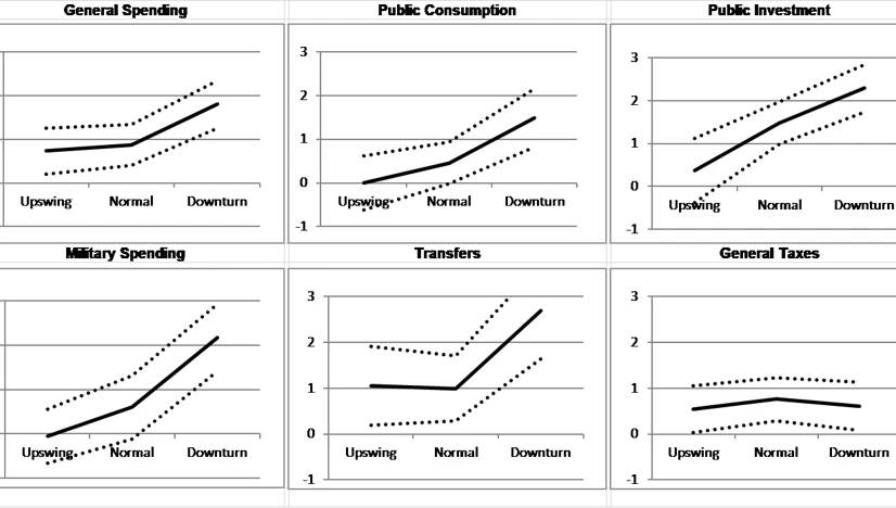
The empirical literature on the multiplier effect has grown significantly since 2007. This is primarily due to two important economic events: the economic stimulus packages around the world to support the economy during the financial crisis and the austerity measures thereafter - especially in the Euro Area since 2010. A 2018 quantitative meta-study (to which the author of this text also contributed) of 98 empirical studies that offer over 1800 estimates of the fiscal multiplier finds large spreads for the multiplier values. At the same time it highlights a few key findings: expenditure side measures have a multiplier effect of 0.8 after 2 years on average, which tends to be higher than for revenue side measures (approx. 0.7). Significantly higher effects of above one are found for public investment and for expenditure side measures during a downturn. Whereas the multipliers of revenue side measures tend to be influenced only very little by the degree of capacity utilization and the business cycle. Figure 1 offers an overview.
Figure 1: Fiscal multipliers by type of impulse and depending on the business cycle. Thick lines = average values, dotted lines = 95% confidence interval; a flat line signals independence from the business cycle, a steep line shows difference due to the business cycle.
Source: adapted from Gechert and Rannenberg (2018)
That the multiplier is larger on the expenditure side than on the revenue side and that the multipliers are larger during a downturn is not uncontested in the economic literature: Ramey’s literature survey (2019) comes to contradictory findings, but is also more selective in the reviewed studies. She concludes that expenditure side multipliers lie between 0.6 and 1 – also during regular downturns - in deep recessions they may turn out to be larger. On the other hand, she notes greater effects for tax cuts with multipliers from 2 to 3, but only refers to studies that use a specific method of estimation. The simulation study from Caldara and Kamps (2017) that compares different approaches however comes to the same conclusions as the before mentioned meta-study: government expenditure tends to have higher multipliers than tax cuts.
How do these contradictory statements and large range of estimations – especially on the revenue side – come about? There are multiple reasons for this. Uncertainties in measurement and country specific differences are obvious candidates. In addition, there is no perfect method for unambiguous separation of the mutual influences of state budget on economic growth (multiplier) and economic growth on the state budget (budget sensitivity) in the data (the so-called identification or endogeneity problem). Therefore, it is necessary to make assumptions about this relationship that can be wrong and, above all else, different.
Capek and Cuaresma (2019) find in a simulation study that results for the multiplier estimations very much depend on a few rather unsuspicious assumptions. The study has its own problems, because it is based on a comparatively short and volatile data set, which make the results more sensitive to changes in assumptions. Nevertheless, it is correct that politics has to deal with the fact that empirical research will not be able to provide secured state of knowledge for a concrete application case.
Ultimately at least a test of plausibility remains: multipliers above 2.5 should probably be viewed skeptically, because the economy grows so strongly in these cases that associated additional revenues as well as reduced expenditures would imply that the original stimulus completely finances itself. This seems rather implausible in view of the past. On the other side of the spectrum, negative multipliers seem equally implausible, because they would imply that higher government spending or tax cuts would reduce GDP. There is also more evidence in favor of, rather than against, that empirical multiplier effects are larger and longer term in times of economic underutilization – i.e. during economic crises – than was generally assumed by decision makers and influential institutions before the financial crisis. The relevant models of the time presumed an effect of about 0.5 – independent of capacity utilization and impulse type.
How did these model implications come into being and how can the different effects be explained theoretically? To understand this, we will take a short tour through the history of economic thought in the next section.
History of ideas and macroeconomic theory
In the first section, we primarily looked at empirical research. But what theoretical foundation do the estimates have and how has the theory changed over time? The underlying idea of the multiplier principle is old. It goes back to the so called Tableau Économique by Francois Quesnay from 1758: additional government spending creates new jobs and higher incomes, this means additional household income, which in turn stimulates additional consumption (we will, for now, leave out the role of companies). According to the simple version of the theory, this results in further cascades of income and expenditure, which in time peter out, and in the end, equal k times the original impulse; k is the size of the fiscal multiplier.
Richard Kahn and John Maynard Keynes helped popularize the idea in the 1930s (and gave the academic background for Franklin D. Roosevelts New Deal). Still today, almost every introductory lecture into macroeconomics refers to the Keynesian Cross (original by Paul Samuelson 1948) or the IS-LM Model (by John Hicks 1937), in which the multiplier effects play a central role.
In these simple static models, the so-called marginal propensity to consume is decisive for the size of the multiplier effect, i.e. how many cents of an additional Euro in income a household spends. To determine the size, simple estimates of consumption rates were used in early empirical studies: households on average spent 80% of their available income on consumption.
A simple mathematical example results: if the marginal propensity to consume is equal to 0.8 on average, then an additional Euro of government expenditure would equal a multiplier effect of k = 1+0.8+0.8²+0.8³+…=1/(1-0.8) = 5. Every additional Euro of government spending would ultimately generate 5 Euro of additional GDP. Tax cuts that increase the available income in essence function the same way, only that the first-round effect on GDP is missing (the ´1´ in the numerical example). Thus the effect would “just” be k = 0.8+0.8²+0.8³+…=0.8/(1-0.8) = 4.
What seems strikingly logical at first glance, raises a couple of questions upon further examination (not only because the values are so high in comparison to the empirical research). Let´s stay on the macro level for now and arrange the channels of influence, ascending with increasing controversiality between the schools of economic thought:
-
It should be apparent that in an open economy a part of the spending on consumption ends up abroad, i.e. it is spent on imported goods or on holiday, and therefore does not stimulate domestic GDP. The greater the tendency to import, the smaller the multiplier.
-
Additionally, the tax administration partially recoups what they spent with the one hand with the other hand: by means of increasing consumption and income tax revenues, but also through reduced expenditure on social benefits, if new jobs are created due to the stimulus. The larger the government share in GDP, the smaller the multiplier tends to be.
-
It is also crucial how strongly the capacities of the economy under consideration are utilized: can the companies even respond to additional demand by increasing production (and hiring new workers) - or does the impulse only effect prices and therefore does not increase real incomes (price crowding-out)? The lower the capacity utilization, the smaller the price crowding-out is and the higher the multiplier tends to be.
-
Also, a reaction in the interest rate is to be expected in dependence on the rate of capacity utilization: if the economy is booming, additional government demand tends to increase financing interest rates thereby inhibiting consumption and investment demand. This also tends to be the case because monetary policy will then presumably become more restrictive (or accommodate less). In a recession, the interest rate reaction is likely to be less pronounced or could even reverse itself. More on this later.
Assuming realistic orders of magnitude for these channels, then one would expect in a model specified in this way for average economies with underutilized capacities, an expenditure multiplier for state consumption of slightly smaller than one, a tax multiplier that is slightly lower and a multiplier for public investment that is a little higher - because it increases capacities, may stimulate private investment,and thereby lessen price crowding-out at the same time. For large closed economies such as the USA the values will be somewhat higher, for small open economies with independent monetary policy somewhat lower. These effects fit quite well in principle with the empirical values from the first section.
End of story? No, because the underlying behavioral assumptions at the micro level have been repeatedly criticized from the get-go and have changed significantly during the course of the history of economic thought, as described in the next section.
Become part of the community!
Exploring Economics is a community project. As an editor you can become part of the editorial team. You can also join one of the many groups of the international Curriculum Change movement.
From macro to micro: Assumptions about individual behavior and its effect on the multiplier, as well as the Zero Lower Bound
In section 2, we primarily described macroeconomic channels on the multiplier. However, also these macroeconomic effects depend on behavioral assumptions at the level of the household.
The simple Keynesian model from section 2 leaves the question unanswered within which time frame the described expenditure cascades should take place because it only compares timeless states of equilibrium (without the fiscal stimulus vs. with the fiscal stimulus) and the chains of effects do look rather mechanistic. To be able to make relevant statements on economic policy however, for example, if a government stimulus will help in time to cushion an economic downturn, the question of timing is very important. Dynamic versions of Keynesian-Neoclassical-Synthesis models based on the first time series data in the 1960s have attempted to answer this question. These models indicated that a large part of the effects would occur within the first 2 years.
This question of dynamics is also a question that addresses the expectations of the respective private actors. How do households react to higher levels of government activity? In the simple model they stoically follow their consumption pattern: if they have additional income, it is a fixed share that is spent again within the same period (One day? One week? One quarter? One year?). They form adaptive (backward looking) expectations. Is this realistic? Proponents of rational (forward looking) expectations would say: no!
Milton Friedman was a thought leader of these ideas on the formation of expectations and was a formative figure for the Monetarist school of thought. He put forward the permanent income hypothesis in the 1950s according to which households would align expected incomes and expenditures over the course of their entire lives. They would pay less attention to their current income and would rather be keen on achieving an even consumption across their entire lives.
Expected permanent changes in income would already be accounted for and would not change consumption at all. Unexpected temporary increases in income (e.g. in form of consumption cheques to stabilize the business cycle, as practiced in the USA during the financial and Corona crises, or as was the case in Germany with the one-off child bonus in 2009) would be quite negligible for lifetime income and would therefore barely increase short term expenditures. The marginal propensity to consume would be close to zero in the short term.
Only unexpected permanent increases in income would have a strong impact on consumption because they immediately and substantially increase the expected lifetime income and the household would adapt its consumption 1:1 immediately.
However, not even permanent expansive fiscal policy would necessarily lead to high multiplier effects. Monetarists explain this either with a restrictive reaction by the central bank that prevents the high multiplier or due to expansive fiscal policy ultimately only leading to price increases without real welfare effects. In contrast, lower taxes on capital and labor could have higher long-term effects, because they would not distort performance incentives and would hence entail expansion of capacities.
In Keynesian models, but also in Friedman´s, the multiplier effect is primarily described via a consumption demand channel. With rational expectations of the New Classical variety emerging in the 1970s, however, the process is quite different. Accordingly, households optimize over their entire life span between consumption and leisure time (lifetime minus working time). If the government decides to spend more money, this increases the current demand for labor and capital (with initially fixed supply). Wages and interest rates rise. This encourages households to work and save more today (and to have less leisure time and consume less). In these models, the restraint on consumption results from additional demand on the goods market by the state crowding out private consumption demand. De facto, consumption even decreases in the short term, but people work more and invest more, which causes GDP to increase. In the long run, this effect reverses into its opposite and consumption rises, but working time decreases. Since households in these models plan very far in advance the intertemporal interest rate channel has enormous influence. In New Classical theory, the multiplier effect is turned into a supply side effect, that in its simplest variant is positive in the short term, negative in the mid to long term and zero in sum.[2] Tax cuts on distorting taxes are expected in these models to increase incentives to work and save. Thereby, positive effects in the short and long term are presumed, as long as the tax cuts are not offset by other distorting taxes in the future.
The New Keynesian paradigm that emerged during the 1990s started from these New Classical behavioral assumptions. It combined them with frictions that make the adjustment in saving, working, consumption and investment to changes in fiscal policy more sluggish (e.g. staggered price and wage adjustments, set up costs for investments, consumption habits). The result is ultimately a mixture of demand and supply side effects. The outcome is a multiplier effect of about 0.5 for revenue and expenditure side measures (again, the effect is a little larger for public investments that are seen to increase capacities). This was the value most institutions assumed prior to the financial crisis.
Zero Lower Bound
Since the financial crisis, the case of the Zero Lower Bound (ZLB) has increasingly been discussed in the New Keynesian framework – a point under which monetary policy can hardly or not at all push the key interest rate. If the optimal interest rate calculated by these models were to be negative, due to a severe recession, monetary policy could not react to fiscal policy, since the key interest rate would remain at 0% either way. As a result, the restraining effect of the interest rate channel is eliminated, and the multiplier is larger. The multiplier is actually even larger because inflation is higher and therefore at a constant nominal interest rate the actually decisive real interest rate decreases.[3] The effects of the ZLB is for the most part conceivable as a mirror image for expansionary and contractionary fiscal policy.
In the context of the crisis in the Euro Area from 2010 onwards, austerity measures by the state played a major role: although the EZB was already close to the ZLB and did not react further in a stabilizing manner, the countries concertedly switched to austerity policies. Since monetary policy could not decrease the key interest rate any further to cushion the crisis, the consolidating policies are expected to have had larger damaging effects.
The effects of the ZLB, however, are not uncontested. Firstly, there are implausibly large differences depending on whether the fiscal stimulus is limited to the phase of zero interest rates (large multiplier), or if it goes beyond this phase (possibly a negative multiplier). Secondly, monetary policy has developed unconventional measures, such as Quantitative Easing and Forward Guidance that could render the ZLB ineffective or at least lessen its importance.
So, is the interest rate channel powerful and multipliers small after all? This claim is in conflict with the cited empirical macroeconomic research in [part 1] and with many studies at the level of the household, which find strong reactions in consumption even to expected and temporary changes in income. These findings are taken into account in more recent models, as shown in the final section.
Multiplier-theory today
The previous section summarized theoretical discussions up to the financial crisis and the case of the ZLB. However, a few questions remained unanswered: in particular, the models prior to the financial crises estimated a multiplier around 0.5; the empirical research, however, shows that especially in economic crises values over 1 are more realistic.
Many current models, therefore, attempt to develop more realistic alternatives to the model landscape that existed before the crisis, in which the interest rate channel and expected future income play a lesser role. Current household income and assets hereby become more important for consumption decisions. For instance, newer models place greater emphasis on the uncertainty of future income, which leads households to save out of caution and discount more strongly for the future. The expected multiplier is therefore significantly higher.
Alternatively or in addition to, some households may have liquidity constraints (for example poorer households that cannot afford to save or cannot access credit; or upper middle class households whose assets are invested in real estate and are thus illiquid). They must, therefore, base their consumption decisions more strongly on their currently available resources, whereby they show a higher marginal propensity to consume than unrestricted households.
Since these characteristics are not evenly distributed amongst the population and depend on employment status and the income level, redistribution from rich to poor could have a positive net effect. Moreover, it is also possible that demand stabilization through fiscal policy in a crisis could give actors more confidence and even lower interest rates, instead of increasing them.
This would support that multipliers are less restrained by the interest rate channel and the supply side channel loses importance. This also leads back to expenditure side measures tending to have higher multipliers than revenue side measures. All in all, these models are now closer to the original Keynesian multiplier effects but offer more realistic behavioral assumptions and account for a multitude of influencing factors.
Bringing such models to greater maturity for application, to further substantiate them empirically and to equip them with further relevant channels of influence from a pluralist perspective will be a big and interesting joint research project for the coming years. In conclusion, it seems that active fiscal policy is especially effective in times of crisis. Even though supply side factors play a major role in the current Corona crisis (international supply chains, production stops) a substantial government demand stimulus is arguably necessary to kick-start the economy again in the aftermath of the supply side constraints. Thinking further ahead, increased public investment, which has a high multiplier effect even in economically normal times, appears to be an essential element for a sustainable growth strategy.
[1] This, however, depends on additional factors and the critical value can be as low as 0.6. In reverse, values larger than 1 (or larger than 0.6 for that matter) imply that austerity measures can increase the ratio of debt to GDP, as explained here. This happens when the multiplier and budget sensitivity are large enough such that GDP and related tax revenues decrease strongly.
[2] If one additionally assumes that households expect higher taxes in the future, due to the increased government deficit today (so called Ricardian equivalence), then these households expect lower net lifetime income. This negative wealth effect causes permanently higher eagerness to work and save and the multiplier can be slightly positive in sum over time, but the multiplier is already small in the short term.
[3] A similar effect arises independent of the ZLB, when monetary policy is not responsible for the management of the business cycle in a single country, but for an entire currency area. Accordingly, it reacts less strongly to fiscal policy measures in the individual countries; or when the central bank, instead of controlling the business cycle, tries to manage the currency exchange rate with high international capital mobility (compare the traditional Mundell-Flemming-Model).